Blog · May 5, 2026
Reinforcement Learning from First Principles (and the Math You Actually Need)
The one sentence the whole field hangs on: The value of where I am is the reward I just got, plus a discounted value of where I’ll land next.
Every algorithm you’ll meet later (Q-learning, DQN, PPO, RLHF, GRPO) is a variation on that single line. This first post builds the intuition behind it and the five pieces of math you need to read it without flinching. No proofs for their own sake; just the ideas, one clean derivation each, a worked example, and then code.
1. The intuition: a world that rolls dice
Reinforcement learning starts from one uncomfortable fact: the world is uncertain, and “how good” a situation is means “how good on average.”
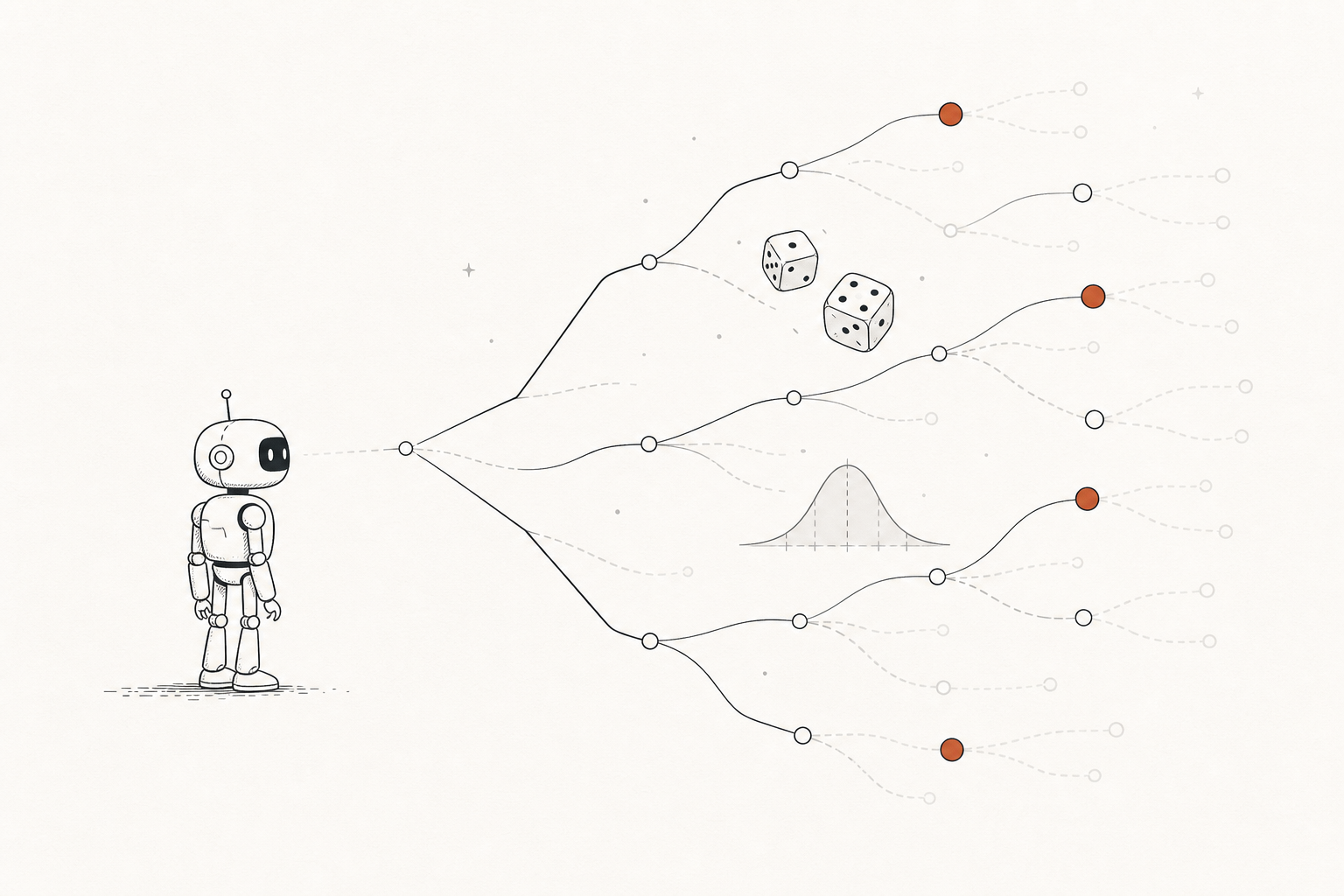
Picture an agent standing at the left of the illustration above. It picks an action and the world branches: maybe the road is clear, maybe it’s jammed; maybe the policy itself flips a coin. You cannot know which branch you’ll get. So you cannot score a situation by a single outcome; you score it by the average over all the branches, weighted by how likely each one is. That average has a name (the expectation), and estimating it from experience is, quite literally, the entire field in one sentence.
The five moving parts
RL describes a loop between an agent and an environment:
flowchart LR
  agent["Agent (policy π)"]
  env["Environment"]
  agent -->|"action a"| env
  env -->|"reward r, next state s'"| agent
At each step the agent observes a state, picks an action from its policy, and the environment answers with a reward and a new state. First, the three primitives of the loop:
- Environment: everything outside the agent. It receives an action and responds with a reward and a new state. The agent cannot change the environment’s rules; it can only choose actions and observe what comes back. A board game, a physics simulator, a web-page layout engine, or a user responding to a chatbot are all environments.
- State (): a complete description of the situation at one instant, containing everything relevant to what happens next. In chess it’s the board position plus whose turn it is; in a self-driving car it might be positions and velocities of every nearby object. In practice the agent often receives an observation () instead, a partial or noisy view of the true state (a camera image, a single Atari frame). When the observation doesn’t capture the full state, the problem is partially observed, and the agent must infer or remember what’s missing.
- Action (): whatever the agent can do at a given step. Actions can be discrete (left, right, stay) or continuous (apply 3.7 N of force at 12° to the left). The set of all available actions is the action space.
Four higher-level concepts build on these:
- Policy (): the agent’s behavior. A map from states to actions (or to probabilities over actions). It can be a lookup table, a neural net, or a search. The policy alone determines behavior. It may be deterministic (“always go left”) or stochastic (“left with 70% probability”).
- Reward signal (): a single scalar each step that defines the goal. The agent’s sole objective is to maximize total reward over the long run. Crucially, reward says what to achieve, not how.
- Value function ( or ): what’s good in the long run. Reward is immediate; value is the total reward you expect to accumulate from here on. A state can have low reward but high value (a boring job that leads to a great career), or high reward but low value (dessert first: great now, hungry later). We act on values, not rewards.
- Model: an optional internal mimic of the environment. Given a state and action, it predicts the next state and reward. With a model you can plan. Without one you must learn from pure trial and error.
2. The math you actually need
Five ideas. Each one shows up in every algorithm later.
2.1 Random variables and expectation
A random variable is a quantity whose value depends on chance. A probability distribution lists each possible value and how likely it is. For a fair die, each of has probability .
The expectation is the long-run average, each outcome weighted by its probability. It’s the center of gravity of the distribution:
For the die, . You never roll a 3.5, but it’s what the rolls average to. This is exactly why value is an expectation, not the result of one lucky run. A single trajectory is one sample from a random process; trust it and you’re fitting noise. Average over all trajectories (weighted by probability) and you get a stable measure of long-term quality.
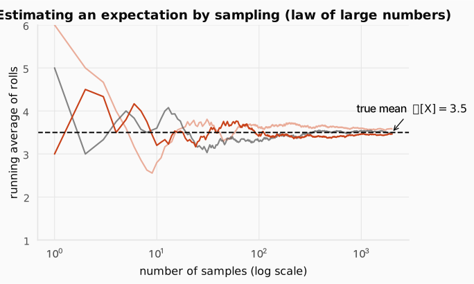
When you can’t compute exactly (because the formula is intractable or you don’t even know the distribution), you estimate it by sampling: draw many samples and average. By the law of large numbers, the sample average converges to the true expectation as you collect more samples (the figure above). The same trick is how an agent will later estimate the expected return (the return is the total discounted reward collected from time onward, ; we make the discounting precise in §2.5): when it can’t compute the average directly, it collects many episodes and averages the returns it actually sees. (That sampling recipe becomes a named method in a later post.)
This is also why estimating value needs no crystal ball. Think of a restaurant you’ve visited three times, twice great and once terrible: you walk in with a gut feeling of “7/10.” That number is the value built from memory, not prophecy, a running average of the returns you actually collected each time you were in state . It reads like a forecast, but nothing here predicts the future; it only averages rewards already observed.
Both routes are one line of NumPy: the exact weighted sum , and the sampled average that converges to it:
import numpy as np
# --- Route 1: Exact expectation via the formula E[X] = Σ x·p(x) ---# faces = [1, 2, 3, 4, 5, 6], each with equal probability 1/6.# Multiplying element-wise and summing gives the true mean: 3.5.faces = np.arange(1, 7)probs = np.full(6, 1 / 6)exact = (faces * probs).sum()
# --- Route 2: Monte-Carlo estimate (sample average → true mean by LLN) ---# We can't always compute E[X] analytically (environments are complex).# Instead, draw N samples and average them.  The Law of Large Numbers# guarantees this converges to E[X] as N → ∞.rng = np.random.default_rng(0)samples = rng.integers(1, 7, size=100_000)   # 100k simulated die rollsestimate = samples.mean()                     # sample average ≈ 3.5
# Both routes should land near 3.5; the gap shrinks with more samples.print(f"exact={exact:.4f} estimate={estimate:.4f}")exact=3.5000 estimate=3.4980The exact weighted sum lands on 3.5; the sampled average from 100 000 rolls lands within 0.002 of it, the law of large numbers at work.
Check: Why is value defined as an expectation over returns rather than the return of a single rollout? What goes wrong if you trust one trajectory?
Answer. A single rollout is one sample from a random process (a stochastic policy and/or environment); it can be very lucky or very unlucky. Value is the mean over all such rollouts. Trust one trajectory and you fit noise: the estimate has huge variance and can be arbitrarily wrong.
Worked example: expectation of a die
2.2 Conditional probability and the Markov property
Conditional probability is “the probability of given that happened.” Knowing can change the odds of .
A process has the Markov property when the next state depends only on the current state and action, not on the entire history:
This isn’t a restriction on the world: it’s a restriction on what counts as the state. The state must include everything relevant. If velocity matters (an Atari ball’s direction), stack a few frames so velocity is in the state. The payoff: the Markov property is what lets us write as a function of alone. If value depended on the whole past, it could never be a simple lookup on the present.
Check: A single Atari frame is not Markov. Why not? What's the standard fix, and what does that fix teach you about the word "state" in general?
Answer. A single frame shows position but not velocity, so you can’t tell which way the ball is moving: the future isn’t determined by the present frame alone. The standard fix is to stack the last few frames. The lesson: “state” isn’t “what you observe,” it’s “whatever makes the future independent of the past.” You engineer the state until the Markov property holds.
Check: Give a real task where the Markov property is badly violated. How would you enlarge the state so it holds again, and what does that cost you?
Answer. Almost any partially-observed task: poker (you can’t see opponents’ cards) or a robot with a narrow camera. Enlarge the state by adding history or a belief over the hidden part. The cost: a much larger state space, more to learn, and you can never inject information that is genuinely unobservable.
2.3 Variance, standard deviation, and the z-score
Expectation is the center; variance is the spread. It measures how far outcomes typically land from the mean:
The z-score re-expresses a value as “how many standard deviations above or below the mean it is”:
This isn’t trivia: the z-score is the heart of GRPO (the algorithm behind modern reasoning models), which you’ll meet in a later post. There, each sampled return is scored relative to its group using exactly this z-score, with the group’s own mean and standard deviation as the baseline. For now the takeaway is just the tool itself: the z-score turns a raw number into “how many standard deviations from the mean.”
Worked example: a z-score from four rollouts
Four rollouts score returns . Compute the mean, standard deviation, and the z-score of the rollout that scored 8.
Mean:
Variance and standard deviation:
Z-score of the rollout scoring 8:
It scored about standard deviations above its group’s average, so its z-score is positive. This same z-score is the quantity GRPO will later use to rank rollouts against their own group; we’ll get to that in a future post.
2.4 The running (incremental) average: the shape of every RL update
You can update an average one sample at a time without storing all the data. Nudge the old estimate a small step toward each new observation:
Read the pieces: is your current belief, is how wrong it was, and is how much you care about the new data. This is the template for every learning rule in reinforcement learning. Monte Carlo, TD learning, Q-learning, actor-critic: all are this nudge applied to slightly different targets.
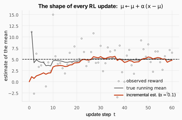
In its RL form, the “new data” becomes a reward-based target and becomes a value estimate, and you’ll see over and over.
Worked example: one incremental-average step
Belief , new observation , step size :
You nudged your belief 10% of the way toward the surprise. Repeat forever: that’s learning.
2.5 Geometric series and discounting
A future reward is worth less than the same reward now. We encode that with a discount factor and weight a reward steps away by . Two consequences fall out of one classic sum. The geometric series
converges because each term shrinks fast enough. That’s why an infinite stream of future rewards adds up to a finite number; otherwise “total future reward” would be meaningless for a task that never ends.
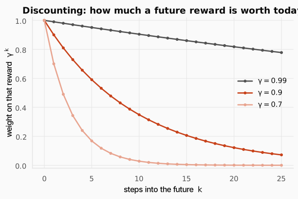
- : completely myopic, only the very next reward matters.
- : far-sighted, distant rewards weigh almost as much as immediate ones.
- : a reward 10 steps away is worth of face value; 50 steps away, .
Check: The return adds up infinitely many rewards. Could it blow up to infinity? Why does γ < 1 prevent that?
Answer. No, as long as . Each step counts a little less than the one before, so the rewards form a shrinking geometric sum. If every reward is at most , then . That bound is the whole reason matters.
Check: Describe, in one sentence each, the agent you get with γ = 0 versus γ = 0.999. When would a low γ actually be the right choice?
Answer. gives a purely myopic agent that maximizes only the immediate reward and ignores all consequences. gives a far-sighted agent that weights rewards hundreds of steps away almost equally. A low is right when the task truly is immediate (one-step decisions) or when long horizons add only noise and instability.
Worked example: discounting adds up to a finite number
With , an endless stream of reward per step is worth
A never-ending task collapses to the number 10. That’s discounting earning its keep.
2.6 Information theory: entropy and KL divergence
The last two tools power every modern policy-gradient method (PPO, TRPO, GRPO). Both are built from a single idea, so we’ll derive that idea once and reuse it.
The problem: measuring uncertainty
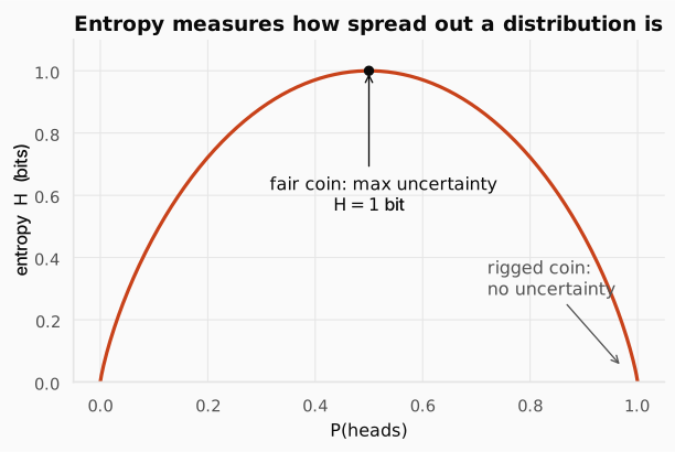
You have a probability distribution (a list of outcomes and their probabilities) and you want one number that answers: how uncertain is this? Two extremes are obvious. A fair coin (50/50) feels maximally uncertain. A rigged coin (100/0) has no uncertainty at all. We need a formula that captures everything in between. It starts with a more basic question: how surprising is a single outcome?
Step 1: Surprise (how much an outcome tells you)
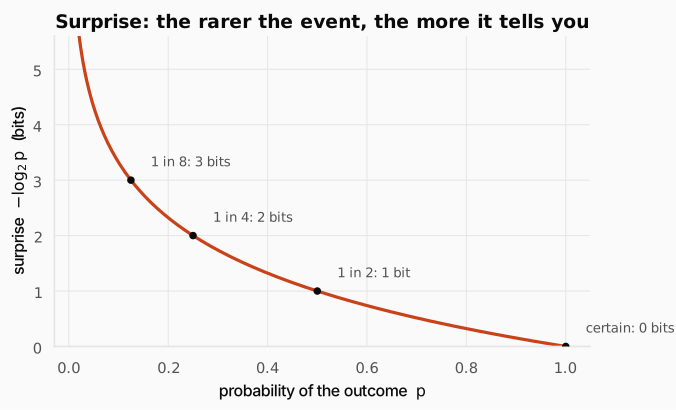
“The sun rose this morning” has probability ; hearing it tells you nothing: zero surprise. “An earthquake hit this morning” has tiny probability; hearing it is a huge shock: large surprise. So surprise should be a function of probability that is large when is small and zero when .
Which function? We want three properties:
- Surprise decreases as increases: likely things are unsurprising.
- An outcome with has zero surprise: certainty tells you nothing.
- Independent surprises add up. Seeing two independent outcomes should sum their surprises, while their joint probability multiplies (). The one function that turns multiplication into addition is the logarithm: .
The unique function satisfying all three is the negative log-probability:
Using measures surprise in bits: bits, bit, bits.
Step 2: Entropy (the average surprise)
Entropy is just the expected surprise: how surprised you should expect to be, on average, before the outcome is revealed. Take the expectation of under itself:
That’s the entire derivation: surprise is ; entropy is its average.
Step 3: What the number tells you
Entropy is high when the distribution is spread out: many outcomes are plausible, so on average you’re quite surprised by what happens. Entropy is low when the distribution is concentrated: one outcome dominates, so you’re rarely surprised. Entropy is exactly zero when one outcome has probability 1, with no uncertainty at all.
Step 4: Why RL cares about entropy
A policy is a probability distribution over actions, so it has an entropy. If the entropy is high, the policy is spread across many actions: it’s exploring. If the entropy is near zero, the policy has collapsed onto a single action: it’s fully committed.
The danger: an agent might collapse too early, before it has gathered enough experience to know which action is truly best. To prevent this, many RL algorithms add an entropy bonus to the reward: a small extra reward for keeping the policy spread out, which encourages the agent to keep trying different actions rather than locking in prematurely.
Step 5: KL divergence (how different are two distributions?)
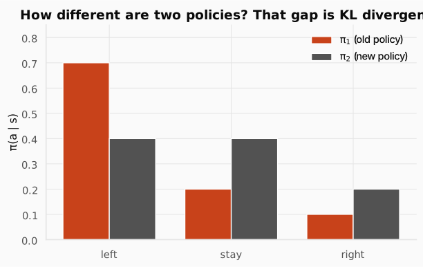
Entropy measures the uncertainty of one distribution. But often we have two and want to ask: how different are they? In RL this is constant: you had a policy , you updated it, and now you have : how much did it change?
Build it from surprise once more. Suppose the world really follows , but you describe it using . For an action , the surprise you actually incur using is , while the smallest (true) surprise was . The extra surprise from using the wrong distribution is
Average that extra surprise over the actions actually produces, and you get the Kullback–Leibler divergence:
It’s the expected number of extra bits you pay for believing when the truth is . Two properties fall right out: always, and iff the two distributions are identical (no extra surprise, nothing wasted).
Why “from ‘s perspective”? Notice the expectation is subscripted with , not : you weight by ‘s probabilities. You’re asking: “for the actions that actually cares about, how differently does treat them?” This is why order matters:
because who does the weighting changes the answer (we’ll see the two numbers differ in the worked example below).
Step 6: Why RL cares about KL
When you update a policy, you want it to get better. But if it changes too much in one step, it can jump to something terrible and never recover. KL divergence measures how far the new policy has drifted from the old one. TRPO, PPO, and GRPO all do the same thing conceptually: don’t let the KL between the old and new policy get too big. It’s a leash: the policy can improve, but it can’t sprint off in a completely different direction in a single update.
These two tools (the z-score from §2.3 and the KL here) both reappear in GRPO in a later post; we’ll see exactly how they fit together when we get there.
Worked example: entropy of a biased coin
A coin lands heads with probability . Its entropy (in bits) is
Compare the extremes: a fair coin gives bit (maximum), and a rigged coin () gives bits. Our biased coin sits in between, closer to certain than to fair, exactly the “everything in between” we wanted to measure.
Worked example: KL divergence between two policies (and why order matters)
Two policies over actions (the figure above):
Forward, extra surprise from ‘s perspective:
Reverse, now weighted by :
Same two policies, different answers (), because whoever does the weighting changes the question. Both are positive and small: is a modest update away from , the kind of step a KL leash would happily allow.
3. Putting it all together: the agent–environment loop in Gymnasium
We’ve mapped each idea to code right where it was introduced. Here’s the whole vocabulary in one place as a quick reference, then a single runnable program that uses all of it at once.
| Concept | Math | In code |
|---|---|---|
| Expectation | (values * probs).sum() | |
| Estimate by sampling | np.mean(samples) | |
| Return (discounted) | G += (gamma ** k) * r | |
| Incremental update | mu += alpha * (x - mu) | |
| Policy | action = policy(state) | |
| Entropy | -(p * np.log2(p)).sum() | |
| KL divergence | (p1 * np.log2(p1 / p2)).sum() |
Gymnasium is the standard RL environment API. Every environment exposes the exact loop from Section 1: reset() gives a starting state, and step(action) returns (next_state, reward, terminated, truncated, info). Below we run a random policy on FrozenLake and estimate the value of the start state (the expected discounted return) by sampling many episodes and averaging. It is the whole post in one function: the loop (§1), the discounted return (§2.5), and estimating an expectation by sampling (§2.1).
import gymnasium as gymimport numpy as np
def estimate_start_value(episodes=20_000, gamma=0.99, seed=0):    """V(start) under a random policy = average discounted return over episodes."""
    # FrozenLake: 4×4 grid, agent must reach the goal without falling in holes.    # ASCII diagram of the environment:    #    #    S  F  F  F    #    F  H  F  H    #    F  F  F  H    #    H  F  F  G    #    # S = Start, F = Frozen (safe), H = Hole, G = Goal    #    # is_slippery=True makes it stochastic (agent slides with probability 2/3),    # so even repeating the same actions can produce different outcomes — a true MDP.    env = gym.make("FrozenLake-v1", is_slippery=True)
    rng = np.random.default_rng(seed)
    # We'll collect one discounted return G per episode, then average them all.    # That average is our Monte-Carlo estimate of V(start) = E[G_t | s₀].    returns = []
    for ep in range(episodes):        state, _ = env.reset(seed=int(rng.integers(1 << 31)))
        # G is the discounted return for this episode (G_t = Σ γ^k r_{t+k+1})        # discount = γ^k, the weight for the k-th future reward; starts at 1        G, discount, done = 0.0, 1.0, False
        # --- The agent–environment loop from §1 ---        while not done:            action = env.action_space.sample()          # random policy π (uniformly random)            state, reward, terminated, truncated, _ = env.step(action)
            # Build the return incrementally: G += γ^k · r_k            # Each reward is discounted by how far into the future it occurs.            G += discount * reward            discount *= gamma                           # γ^k → γ^(k+1) for next step
            done = terminated or truncated
        returns.append(G)
    env.close()
    # Value estimate by sampling: V(s₀) ≈ (1/N) Σ Gᵢ    # std tells us how noisy a single episode is (high variance from §2.3)    return np.mean(returns), np.std(returns)
mean_return, std_return = estimate_start_value()print(f"V(start) ≈ {mean_return:.4f} (std of returns = {std_return:.4f})")V(start) ≈ 0.0121 (std of returns = 0.1031)V(start) ≈ 0.01: under a random policy, only about 1 in 100 episodes reaches the goal (the only source of reward), so the average return is tiny. The standard deviation (~0.10) is about 10x that mean, which tells you that any single episode is almost pure noise: it will return either 0 (fell in a hole) or ~1 (reached the goal), both wildly far from the true average 0.01. You need thousands of episodes before the sample mean settles near the true value.
A few things to notice, each tying straight back to the math:
G += discount * rewardis the discounted return from Section 2.5.np.mean(returns)is estimating the expectation by sampling (Section 2.1).- The large
std_returnis exactly the high variance of Section 2.3: a single episode is a noisy sample, which is why we average thousands. (It’s also the reason Monte Carlo methods are noisy, a thread we pick up in a later post.) - The random
env.action_space.sample()is a (very bad) policy . Replacing it with a good policy (one that maximizes this expected return) is the entire control problem ahead of us. terminatedmeans the episode ended because the environment reached a natural end state (the agent fell in a hole or reached the goal).truncatedmeans the episode was cut short by an external time limit or by reaching a maximum number of steps, not because the task finished. Both end the loop, but they mean different things: a terminated episode’s return is complete, while a truncated episode’s return is artificially shortened.
Run it with
uv run python script.py(orpip install gymnasium numpyfirst). FrozenLake’s only reward is for reaching the goal, so under a random policyV(start)is small, since most episodes fall in a hole and return 0. That small, noisy number is your first value estimate.
Where this goes next
You now have the vocabulary (policy, reward, value, model) and the five tools (expectation, the Markov property, variance, the incremental update, and discounting). The next post formalizes the environment as a Markov Decision Process and derives the Bellman equation, the precise, recursive version of the one sentence at the top:
After that, we’ll meet the three ways to actually solve it (Dynamic Programming, Monte Carlo, and Temporal-Difference learning) and watch all three converge to the same value function on a Gymnasium environment we build from scratch.